Début de la boite de navigation du chapitre
fin de la boite de navigation du chapitre
En raison de limitations techniques, la typographie souhaitable du titre, «
Intégration de Riemann : Intégrale et primitives
Intégration de Riemann/Intégrale et primitives », n'a pu être restituée correctement ci-dessus.
Le calcul de primitive est l'opération inverse du calcul de dérivée.
Début de l'exemple
Exemple
La fonction  a pour primitive sur
  la fonction
 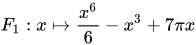 .
.
Pour trouver ce résultat, on lit le tableau des dérivées « en sens inverse » ou on utilise le tableau de primitives ci-dessous.
Fin de l'exemple
On a les propriétés suivantes en utilisant les propriétés de la dérivation :

|
Attention !  n'est pas une primitive de n'est pas une primitive de  , car sa dérivée est , car sa dérivée est  , qui n'a aucune raison d'être égale à , qui n'a aucune raison d'être égale à  . .
|
Contre-exemple : Soient les fonctions  et
et  .
On montre facilement que
.
On montre facilement que 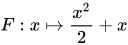 et
et  sont des primitives respectivement de
  et
et  mais pourtant :
1/ 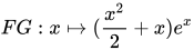 n’est pas une primitive de puisque
 ;
;
2/  est une primitive de car :
 .
.
Soient  des constantes et
  un entier relatif.
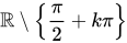
Tableau des primitives simples

|

|

|

|
|

|

|
|
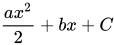
|
 ( ( ) )
|
 si si  ; ;  sinon sinon
|

|

|
|

|

|
|

|

|
|

|

|
|

|

|
|

|

|
|

|

|
|

|

|

|

|

|
|

|

|
|

|
Voici maintenant le lien entre l'intégration et les primitives :
Début d’un théorème
Fin du théorème
Remarques :
- Dans la première partie du théorème, la variable
 est la « borne d’en haut » de l'intégrale : c’est pour cela qu'on parle parfois de « l'intégrale fonction de la borne d’en haut ».
- Ce théorème montre que toute fonction continue admet des primitives.
Démonstration
- Notons
 la fonction
 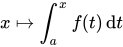 Il est clair qu'elle s'annule en
  :
: 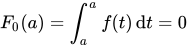 .
.
Il faut montrer maintenant que est bien une primitive de , c'est-à-dire que  ou encore (par définition de la dérivée) que

La relation de Chasles donne :

donc :

Soit  . Par continuité de au point
  , il existe
  tel que
![{\displaystyle \forall t\in [x_{0}-\eta ,x_{0}+\eta ]\quad |f(t)-f(x_{0})|\leq \varepsilon }](https://wikimedia.org/api/rest_v1/media/math/render/svg/b084e6da05072321f8ffaa74b8ef4c40dff62922)
donc tel que
![{\displaystyle \forall x\in [x_{0}-\eta ,x_{0}+\eta ]\quad \left|{\frac {F_{0}(x)-F_{0}(x_{0})}{x-x_{0}}}-f(x_{0})\right|\leq {\frac {1}{x-x_{0}}}\int _{x_{0}}^{x}\left|f(t)-f(x_{0})\right|\,\mathrm {d} t\leq \varepsilon }](https://wikimedia.org/api/rest_v1/media/math/render/svg/0182edba15e36c6ae658724c99a766147e0490e2) : c’est précisément ce qu’il fallait démontrer.
: c’est précisément ce qu’il fallait démontrer.
- Toute primitive de est de la forme
 pour une certaine constante
  , donc
 , ce qui est le résultat annoncé.
Exemples :
![{\displaystyle \int _{0}^{1}x^{2}\,\mathrm {d} x=\left[{\frac {x^{3}}{3}}\right]_{0}^{1}={\frac {1^{3}}{3}}-{\frac {0^{3}}{3}}={\frac {1}{3}}.}](https://wikimedia.org/api/rest_v1/media/math/render/svg/51f8acf6b627f18f9705cad5d2dae76296176c60)
![{\displaystyle \int _{2}^{5}x^{2}\,\mathrm {d} x=\left[{\frac {x^{3}}{3}}\right]_{2}^{5}={\frac {125}{3}}-{\frac {8}{3}}={\frac {117}{3}}=39.}](https://wikimedia.org/api/rest_v1/media/math/render/svg/82ff04a1f38791f0d77753807c36983c177353d0)
![{\displaystyle \int _{0}^{1}\mathrm {e} ^{2x}\,\mathrm {d} x=\left[{\frac {1}{2}}\mathrm {e} ^{2x}\right]={\frac {\mathrm {e} ^{2}-1}{2}}.}](https://wikimedia.org/api/rest_v1/media/math/render/svg/88f6a4846356d1f1204814e16795a452de456663)
Notion d'intégrale indéfinie (sans bornes) :
Soit une fonction définie sur un intervalle  admettant des primitives.
On note  , l'ensemble de toutes les primitives de sur l'intervalle .
Donc, si  est une primitive de sur :
Par abus de langage, cette notation désigne aussi une primitive quelconque de : il faut toutefois bien garder à l'esprit qu’il existe une infinité de primitives définies à une constante additive près.
La principale méthode utilisée pour calculer des intégrales est d’abord l'usage du théorème fondamental de l'analyse.
Notez qu'on n'utilise (presque) jamais la définition théorique de l'intégrale pour calculer une intégrale.
Début d’un théorème
Fin du théorème
Démonstration
Il suffit d’utiliser la formule de dérivation d'un produit :
![{\displaystyle (uv)'=u'v+uv'\Rightarrow u'v=(uv)'-uv'\Rightarrow \int u'(x)v(x)\,\mathrm {d} x=\left[u(x)v(x)\right]-\int u(x)v'(x)\,\mathrm {d} x}](https://wikimedia.org/api/rest_v1/media/math/render/svg/9685bbb59fd031c4b6eccb0aef3ca7b47bde433c) , d'où le résultat.
, d'où le résultat.
Exemples :
1/ Calculer  .
.
On intègre par parties en posant :


On a donc :
|

|
2/ Une double intégration par parties :
Calculer 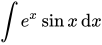 .
.
On intègre par parties en posant :


On a donc :

Pour calculer la dernière intégrale, on intègre (encore) par parties en posant :

On a donc :
 . On est revenu à l'intégrale qu'on voulait calculer : le serpent se mord la queue ! Est-on réellement bloqué pour autant ?
Solution : on retombe sur ses pieds et le serpent garde sa queue !
En fait, il suffit d'« injecter » le résultat obtenu pour
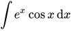
dans le résultat obtenu dans la première intégration par parties ; on obtient :

Il suffit alors d'ajouter de chaque côté et l’on a :
 , d'où l’on tire :
|

|
3/ Calculer 
On ne connaît pas a priori de primitive de  (et c’est bien ce qu'on cherche).
L'astuce dans ces cas-là (une fonction « seule » dont on ne connaît que la dérivée mais pas la primitive) consiste à intégrer par parties en posant :
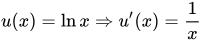
 .
.
(On a remarqué que  , tout simplement !)
On a donc :

Donc (c'est un résultat à retenir) :
|
 . .
|
On montre en fait plus généralement (et sans plus de difficulté) que pour tout réel  :
:

:
Début d’un théorème
Fin du théorème
Démonstration
Il suffit d’utiliser la formule de dérivation d'une composée :
 , d'où le résultat par intégration.
Remarque : Une fonction  bijective de classe
  dont la réciproque est alors de classe est appelée un -difféomorphisme.
Pour utiliser cette formule en pratique :
- poser
 et donc
 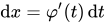 ;
;
- changer les bornes d'intégration : si
 , alors
  et si
et si 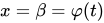 , alors
  .
.
Remarquez que cette formule s'utilise dans les deux sens, comme le montrent les exemples.
Exemples :
1/ ![{\displaystyle \int _{1}^{2}{\frac {x+2}{x^{2}+4x-1}}=\int _{4}^{11}\,{\frac {\mathrm {d} t}{2t}}=\left[{\frac {1}{2}}\ln t\right]_{4}^{11}={\frac {\ln 11-\ln 4}{2}}}](https://wikimedia.org/api/rest_v1/media/math/render/svg/d50dbf7adac40fe49a2392de15a4fb0cf2cf11a2) .
.
On a fait le changement de variables  et
et  .
.
Pour les bornes : si  , alors
  et si
et si  , alors
  .
.
2/  puisque
  .
.
On pose  donc
donc  .
.
Alors  à une constante près.
On a posé  et donc
  .
.
Pour intégrer une fraction rationnelle (si la solution ne peut être trouvée directement avec les méthodes ci-dessus), il faut la décomposer en éléments simples . L'intégration devient ensuite relativement aisée sauf lorsqu'on rencontre des éléments simples de deuxième espèce de la forme :
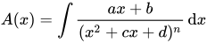 où
où  et
et  .
.
Pour calculer  , il faut :
1/ Faire apparaître la dérivée du dénominateur au numérateur :
 .
La seule réelle difficulté qui est apparue est le calcul de
.
La seule réelle difficulté qui est apparue est le calcul de 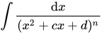 . C'est ce calcul que l’on va chercher maintenant à effectuer.
2/ Remplacer  par sa forme canonique :
On obtient  .
.
On cherche à calculer  .
.
3/ Calculer 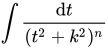 :
:
- Si
 , alors on obtient
 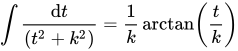 (voir « fonction arctan »).
- Si
 , alors on pose
 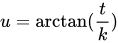 et l'on a (tous calculs faits…) :
 , qu'on calcule par linéarisation avec les formules d'Euler.
Voir Changement de variable en calcul intégral/Intégrales contenant des fonctions trigonométriques.







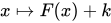




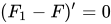









![{\displaystyle [a,b]}](https://wikimedia.org/api/rest_v1/media/math/render/svg/9c4b788fc5c637e26ee98b45f89a5c08c85f7935)

![{\displaystyle \int _{a}^{b}f(x)\,\mathrm {d} x=[F(x)]_{a}^{b}=F(b)-F(a)}](https://wikimedia.org/api/rest_v1/media/math/render/svg/1e249807d9c29c495652b2b5f57d34fefd7193a4)


![{\displaystyle \int _{a}^{b}u'(x)v(x)\,\mathrm {d} x=\left[u(x)v(x)\right]_{a}^{b}-\int _{a}^{b}u(x)v'(x)\,\mathrm {d} x.}](https://wikimedia.org/api/rest_v1/media/math/render/svg/cd0eff99d3644077823fdacf5a1317718634129e)
 Faites ces exercices : Intégration en mathématiques/Exercices/Primitives 4#Exercice 7-3 (niveau 13).





